Least Squares Linear Regression

Least-squares regression is a methodology for finding the equation of a best fit line through a set of data points. It also provides a means of describing how well the data correlates to a linear relationship. An example of data with a general linear trend is seen in the above graph. First, we will go over the derivation of the formulas from theory and then I have also appended at the end of this post Scilab code for implementation of the algorithm.

The equation of a line through a data point can be written as:

The value of any data points that are not directly on the line but are in the proximity of the line can be given by:

Where e is the vertical error between the y-value given by the line and the actual y-value of the data. The goal would be to come up with a line which minimizes this error. In least-squares regression, this is accomplished  by minimizing the sum of the squares of the errors. The sum of the squares of the errors is given by:

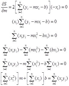
In order to minimize this value, the minimum finding techniques of differential calculus will be used. First take the derivative with respect to the slope.

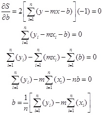
Then with respect to the y-intercept yields:

Which can be substituted in the previous equation to solve for the slope.

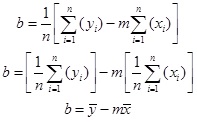
The y-intercept is then:

It can be seen that these last two formulas only require knowledge about the data point coordinates and the number of points and the equation for the least squares linear regression line can be found.

Finally, below is the Scilab code implementation.

//the linear regression function takes x-values and
//y-values of data in the column vectors 'X' and 'Y' and finds
//the best fit line through the data points. It returns
//the slope and y-intercept of the line as well as the
//coefficient of determination ('r_sq').

//the function call for this should be of the form:
//'[m,b,r2]=Linear_Regression(x,y)'
function [slope, y_int, r_sq]=Linear_Regression(X, Y)
    //determine the number of data points
    n=size(X,'r');

    //initialize each summation
    sum_x=0;
    sum_y=0;
    sum_xy=0;
    sum_x_sq=0;
    sum_y_sq=0;

    //calculate each sum required to find the slope, y-intercept and r_sq
    for i=1:n
        sum_x=sum_x+X(i);
        sum_y=sum_y+Y(i);
        sum_xy=sum_xy+X(i)*Y(i);
        sum_x_sq=sum_x_sq+X(i)*X(i);
        sum_y_sq=sum_y_sq+Y(i)*Y(i);
    end

    //determine the average x and y values for the
    //y-intercept calculation
    x_bar=sum_x/n;
    y_bar=sum_y/n;

    //calculate the slope, y-intercept and r_sq and return the results
    slope=(n*sum_xy-sum_x*sum_y)/(n*sum_x_sq-sum_x^2);
    y_int=y_bar-slope*x_bar;
    r_sq=((n*sum_xy-sum_x*sum_y)/(sqrt(n*sum_x_sq-sum_x^2)*sqrt(n*sum_y_sq-sum_y^2)))^2;

    //determine the appropriate axes size for plotting the data and
    //linear regression line
    axes_size=[min(X)-0.1*(max(X)-min(X)),min(Y)-0.1*(max(Y)-min(Y)),max(X)+0.1*(max(X)-min(X)),max(Y)+0.1*(max(Y)-min(Y))];

    //plot the provided data
    plot2d(X,Y,style=-4,rect=axes_size);

    //plot the calculated regression line
    plot2d(X,(slope*X+y_int));
endfunction

I hope this proves helpful. Let me know in the comments if you have any questions.

Related Posts:

Maximizing and Minimizing

The Bisection Method Using Scilab

Structural Finite Element Analysis Software Installation

The Bisection Method using Scilab

 

Recently, I have really been enjoying learning to use Scilab which is an open-source mathematics software that works alot like Matlab. Specifically we have run into some design problems in water and wastewater engineering that involved solving for variables that are described implicitly by an equation and cannot be solved through typical algebraic means. For example:

This cannot be solved directly for x. So how can we find the value of x that will satisfy the equation? Well this is where the numerical analysis technique of the bisection method comes in. The bisection method is a bounded or bracketed root-finding method. In other words, it will locate the root of an equation provided you give it the interval in which a root is located.

The search for the root is accomplished by the algorithm by dividing the interval in half and determining if the root is in one half or the other. Then it divides that interval in half and so on until it gets within a specified relative error. Below I have entered my code for this algorithm. If you save this file as Bisection_Method.sci in a scilab/modules/…/macros folder and execute it in the SciNotes editor, you can then use it by entering a command in the console like:

root = Bisection_Method(‘x-sinx-3’,0,6.5,0.5)

The first passed parameter is the function equation itself solved such that f(x) = 0. The second parameter is the lower end of the interval while the third is the upper end. The final parameter is the percent relative error that the algorithm much reach with the solution before it terminates and gives a result.

Please feel free to download Scilab for free here and copy this code and use it. Let me know if you have any troubles or if you find a problem with the code.

 

//The Bisection Method is a bracketed root locating method. Therefore
//the user must input the lower and upper bounds on the interval where
//the root is to be located. 
//func_expression - must be a string containing the function expression
//with the variable written as 'x'.
//es - is the relative percent error criterion that must be met for the
//method to terminate.
function [root]=Bisection_Method(func_expression, x_lower, x_upper, es)
    x = x_upper;
    fu = evstr(func_expression); //evaluate the function at x_upper
    x = x_lower;
    fl = evstr(func_expression); //evaluate the function at x_lower
    //***********************************************************
    //test to see if there is a root in the interval
    if (fu*fl >= 0) then
        root = 'no root in interval given';
    else
        //there is a root in the interval
        exact_solution = 'notfound';
        ea = 100;
        xr_new =(x_upper + x_lower)/2;
        //*******************************************************
        //iteratively progress toward to root until it is found or it
        //is approximated with a relative error less than required
        while ea > es & exact_solution == 'notfound',
            x = xr_new;
            fr = evstr(func_expression);
            x = x_lower;
            fl = evstr(func_expression);
            //***************************************************
            if(fl*fr < 0) then
                x_upper = xr_new;
            elseif(fl*fr > 0) then
                x_lower = xr_new;
            elseif(fl*fr == 0) then
                root = xr_new;
                exact_solution = 'found';
            end //of if statement
            //***************************************************
            //calculate the approximate relative error for the iteration
            xr_old = xr_new;
            xr_new =(x_upper + x_lower)/2;
            ea = abs((xr_new - xr_old)/xr_new)*100;
        end //of while loop 
        //*******************************************************
        //if error criterion has been met but the exact answer has not
        //been found, set the root to the adequate approximation.
        if (exact_solution == 'notfound') then
            root = xr_new;
        end //of if statement
        //*******************************************************      
    end //of if-else statement
    //***********************************************************
endfunction